Accessible spreadsheets

We use Spreadsheets to present tabular data. This guide will help you to create them more accessible.

Content

Styles and Headings
Add content to cell A1
Hyperlinks
Images and Alternative Text
Colour contrast
Use of colour
Tables
Delete empty rows/columns
Avoid splitting or merging cells
Create a table for your data
Name the table
Use table headers
Accessibility Checker
Name worksheets
Remove blank sheets
Hide unused cells
Name workbook
Further reading

Styles and Headings

Make sure the spreadsheet headings are created using Heading styles rather than using a big, bold font.

Use Microsoft Excel's styles from the Styles group of the Home tab. Use Heading 1 for the main heading, use Heading 2 for section headings, and Heading 3 for sub headings within sections. Heading styles can be found from

Home > Styles > Titles and Headings

Add content to cell A1

Screen readers start reading content from cell A1. By having content in cell A1 makes it easier for users with site impairments to navigate and orientate.

Hyperlinks

Include meaningful hyperlinks in your document. Each hyperlink in your text should convey relevant information about the destination of the link.

Images and Alternative Text

It is essential that you add alt text to each image, chart, graph, or other non-text elements. If you miss alt text, screen reader users will hear the word “image” but not know what the image is. However, if your image has no meaning, the image menu would give you the option to mark the image as decorative.

Right click on the image and select "View Alt Text ..." to open the Alt text panel. Here you can either provide a description or mark the image as decorative as appropriate.

Colour contrast

Use sufficient colour contrast between text and background to make it easier to read.

Useful link

Learn more about colour contrast

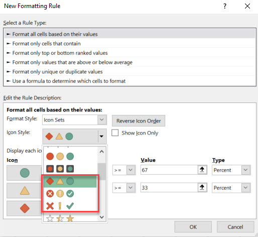
Use of colour

Do not use colour as the only way to represent information. It is common practice to format cells based on their values. When you are formatting, use a scheme where both colour and a shape is used to differentiate content.

Useful links

Accessible use of colour

Tables

Do not rely on borders to show a table as this information will not be conveyed to screen reader users. Instead, you can create tables for your tabular data. This will not only make your worksheet more accessible, but it will also allow you to sort and filter data in your table. You can use Table Design to style your table.

Delete empty rows/columns

When you have data in tabular format if there are empty rows or columns in between, arriving at an empty row/column a screen reader user may assume that the data ends at that point. Deleting the empty rows/columns will avoid this misunderstanding. If you cannot avoid a blank cell, column or row, enter text explaining that it is a blank. Microsoft suggests inserting N/A or Intentionally Blank.

Avoid splitting or merging cells

Screen readers count table cells to keep track of location. When there are nested tables, merged or split cells, the screen reader loses count and can’t provide helpful information about the table after that point. This affects screen reader user's ability to navigate the table. The Accessibility Checker in Excel is able to identify these issues.

Create a table for your data

Select the data range. Select Insert > Table this will give you the Create Table options dialog. Check the cell range to make sure all data is covered. If your table had headers tick the checkbox My table has headers. Now select OK.

If you have not created a table before this Microsoft tutorial on Create and format tables will be a useful guide.

Name the table

By default, Excel names tables as Table1, Table2 and Table3. But to make it easier to refer to a table you can provide a descriptive name to the table. To name the table, place the cursor anywhere on the table. On Table Design tab, under Table Name provide a meaningful name.

Use table headers

Place the cursor anywhere in a table. On the Table Design tab, in the Table Style Options group, select the Header Row checkbox. Type the column headings.

Accessibility Checker

Use Review > Check Accessibility to invoke the accessibility checker. This will help you to identify issues in your worksheet.

Name worksheets

Give all worksheets unique, descriptive name. Screen readers read the sheet names providing information to the user. Giving unique and descriptive names for all worksheets will make it easier for them to navigate the content in the workbook.

Useful links

Rename worksheets

Remove blank sheets

Removing blank worksheets in a workbook allows screen reader users (and everyone else) the ease of navigation.

Useful links

Delete blank worksheets

Hide unused cells

To reduce visual clutter, you can hide the cells that are unused in a worksheet. Go to the last column used and select all cells to the right (in Windows you can use Shift + Ctrl + right arrow). Right click on the selected area and select "Hide" from the popup menu.

Similarly do this for unused rows. In Windows computers select the row below the last row of data and press Shift + Ctrl + down arrow. Right click on the selected area and select "Hide".

Name workbook

Provide a meaniningful name for the workbook. For example, instead of saving the workbook with a generic name such as "Workbook1", provide a descriptive name that describes the purpose of the workbook. This will make it easier to be located for all users.